This post is going to give a brief introduction to deep models, the history of object detection ranging from classic methods based on hand-crafted features to the latest deep learning object detectors, object detection datasets, and object detection evaluation metrics.
Deep Models Preface
The construction of well performing deep models in complex computer vision tasks is often two-fold. The primary goal is to find a model architecture defined by a directed computation graph \(G = \left( V, E \right)\) connecting model inputs \(\left\{ \boldsymbol{X}_{0}, \dots, \boldsymbol{X}_{K_{\mathrm{in}}-1} \right\}\), with \(\boldsymbol{X}_{k} \in \mathbb{R}^{d_{0} \times \dots \times d_{D_{k}-1}}\) to nodes \(v_{i} \in V\) to model outputs \(\left\{ \boldsymbol{Y}_{0}, \dots, \boldsymbol{Y}_{K_{out}-1} \right\}\) with \(\boldsymbol{Y}_{k} \in \mathbb{R}^{d_{0} \times \dots \times d_{D_{k}-1}}\). Each node \(v_{i}\) in the graph represents an operation \(f\) performed on one or more inputs which in turn generates one or more outputs. The operation can be arbitrary as long as it is differentiable w.r.t. each of its input, i.e.
\[\frac{\partial f \left( \boldsymbol{X}_{0}, \dots, \boldsymbol{X}_{K_{in}-1} \right) }{\partial \boldsymbol{X}_{i}},\quad 0 \leq i \leq K_{\mathrm{in}}\] exists. These operations can be mainly divided into two groups. The first group consists of parametric operations, i.e. the operations’ output additionally depends on a set of weights that are adjustable during the optimization step. Prime examples for this group are fully connected layers, which are implemented as affine transformations:
\[f_{linear} \left( \boldsymbol{x} ; \boldsymbol{W}\right) = \boldsymbol{x} \cdot \boldsymbol{W}, \quad \boldsymbol{x} \in \mathbb{R}^{D_{in}}, \quad \boldsymbol{W} \in \mathbb{R}^{D_{\mathrm{in}} \times D_{\mathrm{out}}} ,\] where \(\boldsymbol{W}\) is the weights matrix (with an implicit bias encoding) that maps the input from \(\mathbb{R}^{D_{\mathrm{in}}}\) to \(\mathbb{R}^{D_{\mathrm{out}}}\), as well as convolution layers, implementing the convolution (which is actually a cross-correlation) operation with weight window, also called kernel map, \(\boldsymbol{W} \in \mathbb{R}^{K_{H} \times K_{W}}\), with \(K_{H}\) and \(K_{W}\) odd, over an input \(\boldsymbol{X} \in \mathbb{R}^{H \times W}\):
\[f_{\text{conv2d}, m, n} \left( \boldsymbol{X} ; \boldsymbol{W} \right) = \sum_{i = - \frac{K_{H}-1}{2}}^{\frac{K_{H}-1}{2}} \sum_{j = - \frac{K_{W}-1}{2}}^{\frac{K_{W}-1}{2}} W_{\frac{K_{W}-1}{2} + i, \frac{K_{H} - 1}{2} + j} X_{m-i, n-j} \quad .\] Note that this operation in particular is the 2D convolution often used in image processing which is only one of many possible convolution operations. Other convolution operations that are commonly used include 1D and 3D convolution, as well as convolutions with stride, convolutions with dilations, depth-wise, and separable convolutions. Parametric operations have the additional constraint to be differentiable w.r.t. their weights, i.e. \(\partial f \left( \boldsymbol{X}_{0}, \dots, \boldsymbol{X}_{K_{\mathrm{in} - 1}} ; \boldsymbol{W} \right) / \partial \boldsymbol{W}\) exists.
The second group is formed by non-parametric operations. That is, operations that do not include any learnable weights. Common examples for those are activation functions such as
\[\begin{aligned} \text{sigmoid} \left( x \right) &= \frac{1}{1 + e^{-x}} \\ \text{tanh} \left( x \right) &= \frac{e^{x} - e^{-x}}{e^{x} + e^{-x}} \\ \text{ReLU} \left( x \right) &= \text{max}(0, x) \end{aligned}\] which are usually used after affine transformations to achieve non-linearity. Other common non-parametric operations are pooling, normalization (although some normalization techniques such as Batch Normalization do have learnable parameters), dropout , and softmax.
The second important step in the development of deep models is the choice of a proper loss function. The loss function \(L\), also called a cost function, measures the overall loss of a model \(f\) in taking a decision or action. The goal for the model is to minimize the loss value \(L( \boldsymbol{x}, \boldsymbol{y}, f)\) for some input \(\boldsymbol{x}\) and the apriori known ground-truth target \(\boldsymbol{y}\). This is achieved by computing the gradient of the loss w.r.t. the weights at each node in the computation graph, using backpropagation and optimizing the weights by taking a descent step in the gradient direction. Simple machine learning tasks use single-term loss functions like the cross-entropy loss for classification or some form of distance metric such as the mean-squared-error for regression. Other tasks may require multiple objectives, such as regressing the coordinates of a bounding box and classifying the object inside that box in object detection. Therefore, loss functions can also be composed of multiple objectives, where each objective \(i\) is represented by its loss function \(L_{i}\), weighted by \(\lambda_{i} \in \mathbb{R}^{+}\):
\[L \left( \boldsymbol{x}, \boldsymbol{y}, f \right) = \sum_{i} \lambda_{i} L_{i} \left(\boldsymbol{x}, \boldsymbol{y}, f \right) .\] It is common to include loss terms that are independent of the input and output such as weight decay applying a regularization on the weights, encouraging the model to keep the weights small, as well as gradient penalty which normalizes gradients w.r.t. the inputs, commonly found in successful Generative Adversarial Network architectures.
Quantification of Object Detection Performance
Before we begin to dive into the methodology of object detection, the following will shortly describe common datasets, as well as the de facto standard metric, the mean Average Precision (mAP), in the field of object detection.
Datasets
In computer vision and machine learning in general, the quality of the data which is used to train a model is of utmost importance. The following section lists common datasets for horizontal object detection and oriented object detection.
Horizontal Object Detection
PASCAL VOC
The PASCAL Visual Object Classes (VOC) Challenges (2005 — 2012) includes multiple tasks such as image classification, object detection, semantic segmentation, and action detection. The two most prominent datasets in use for object detection evaluation are VOC07 with 10k training images and 25k annotated objects, and VOC12 with 12k training images and 27k annotated objects. Both datasets contain 20 different classes which are common in everyday life situations such as persons, animals, vehicles, and indoor objects.
ILSVRC
The ImageNet Large Scale Visual Recognition Challenge (2010 — 2017) is a object detection challenge based on the ImageNet dataset. It contains 200 classes and 517k images with 534k annotated objects beating VOC by two orders of magnitude in scale.
COCO
The Common Objects in Context (COCO) (2015 — 2019) is a large-scale object detection, segmentation, and captioning dataset with 80 object categories in 164k images (COCO17) and 897k annotated objects. Before the Open Images Detection challenge (see below), COCO was the most challenging object detection dataset since it contains more object instances per image and more small objects (with a relative image area below 1%), as well as more densely located objects than VOC and ILSVRC.
OID
The Open Images Detection (OID) challenge (2016 – 2020) released the largest object detection dataset to date in 2018, consisting of 1.9M images with 16M annotations across 600 object categories. Due to the dataset being relatively new, only very few papers publish evaluations for OID.
Oriented Object Detection
The task of oriented object detection requires ground-truth orientation labels for each bounding box. For the above-mentioned datasets, these can only be obtained by applying a minimum-bounding-rectangle algorithm on the complex hull of the segmentation map of each object. Alternatively, oriented object detection datasets have been gathered, as listed below.
DOTA
The Dataset for Object Detection in Aerial Images (DOTA) was released as part of the Object Detection in Aerial Images (ODAI) challenge in early 2018. In the first version (1.0) of the dataset, a total of 2806 images are collected from Google Earth and vary in size between \(800 \times 800\) and \(4000 \times 4000\) pixels, annotated by 188k objects in total. Each object instance annotation consists of an arbitrary quadrilateral, i.e. 8 degrees of freedom (four pairs of \(x\)- and \(y\)-coordinates), as well as one label from a set of 15 possible object categories. While all publications on oriented object detection evaluate on version 1.0 of DOTA, the dataset authors have additionally published version 1.5 which introduces an additional class and increases the number of annotations on the existing image base to 403k.
HRSC2016
The High Resolution Ship Collection (HRSC) dataset was collected from Google Earth and consists of 1.7k satellite images. Each image can contain multiple ships and each ship is annotated with a 5-tuple describing the pixel location, width, height, and rotation angle. Additionally, each ship is annotated with a label for the ship class, a specific category, and a ship type.
ICDAR
The International Conference on Document Analysis and Recognition (ICDAR) offers the ICDAR2015 challenge on incidental scene text detection containing 1.7k everyday scene images. Each text instance is annotated with a quadrilateral (8 degrees of freedom) specifying the arbitrary bounding box and the actual text content.
FDDB
The Face Detection Data Set and Benchmark (FDDB) is a dataset of faces, designed to study the problem of unconstrained face detection. The annotations consist of 5.2k faces in 2.8k images, where each instance is described by a 5-tuple of rotated ellipsis.
Measuring Detection Accuracy
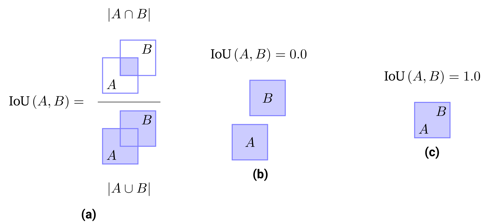
The Intersection over Union metric can be computed by measuring the proportion of the intersection between two bounding boxes w.r.t. their joint area, see (a). The IoU value ranges between $0.0$ when $A \cap B = \emptyset$ (b) and $1.0$ when $A \cap B = A \cup B$, implying that $A = B$ (c).
The most common evaluation metric in object detection is the mean Average Precision (mAP), originally introduced in VOC07. The mAP score is computed as the average object detection precision, i.e. “What proportion of positive detections was actually successful?”, over different recall values, i.e. “What proportion of actual positives was detected successfully?”, evaluated for each object class separately and averaged afterward. The values for precision and recall can be computed as follows:
\[\begin{aligned} \text{Precision} &= \frac{\text{TP}}{\text{TP + FP}} \\ \text{Recall} &= \frac{\text{TP}}{\text{TP + FN}} , \end{aligned}\] where TP is the number of true positives, while FP and FN are the numbers of false positives and false negatives respectively. The natural follow-up question is how a detection match and miss is decided. In a binary classification problem, we simply check for equality between the predicted and the target label. In the setting of object detection, the targets and predictions consist of tuples of coordinates that define a bounding box. Hence it is necessary to define a rule at which point the prediction matches the target box in the two-dimensional image space. This rule can be expressed as a hard threshold for the so-called Intersection over Union (IoU) value which measures the relative overlap between the two boxes \(|A \cap B|\) w.r.t. their common covered area \(|A \cup B|\) (see Figure above):
\[\text{IoU}\left( A, B \right) = \frac{|A \cap B|}{|A \cup B|} .\] The IoU score ranges between a value of 0.0 when there is no overlap between the two boxes (\(A \cap B = \emptyset\), Figure (b)) and 1.0 when the boxes are equal (\(A \cap B = A \cup B\), Figure (c)). For a fixed IoU score threshold \(\tau\), we can now count the necessary statistics to compute the precision and recall values as follows:
-
True Positives: Number of predicted boxes \(A\) that fulfil \(\text{IoU}\left( A, B \right) \geq \tau\) for at least a single target box \(B\), i.e. those objects which are correctly localized.
-
False Positives: Number of predicted boxes \(A\) that fulfil \(\text{IoU}\left( A, B \right) < \tau\) for all target boxes \(B\), i.e. those predictions that did not sufficiently overlap with any target.
-
False Negatives: Number of target boxes \(B\) that fulfil \(\text{IoU}\left( A, B \right) < \tau\) for all predicted boxes \(A\), i.e. those targets that had no sufficient overlap with any prediction.
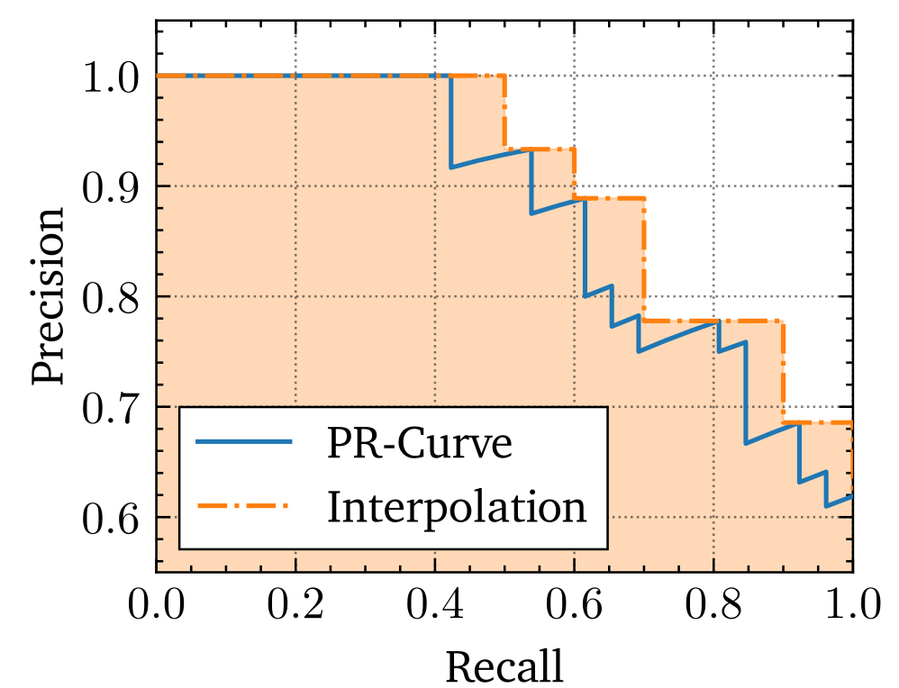
An example precision-recall curve. The blue line represents the true PR-Curve, while the dotted orange line is the 11-point interpolation which at recall point $\tilde{r}$ uses the maximum precision value $p \left( r \right)$ for all $r \geq \tilde{r}$ with $\tilde{r} \in \left\{ 0.0, 0.1, \dots, 1.0\right\}$. The Average Precision score is equal to the area under the 11-point interpolation of the precision-recall curve.
Following a sorting procedure of each prediction based on object classification confidence value, we can then generate the precision-recall curve by counting the number of TP, FP and FN cumulatively along the confidence-ascending list of predictions as shown with the blue line in the above figure. The Average Precision (AP) score reflects the area under the precision-recall curve. To be more robust against small changes in prediction confidences and the following change in the precision-recall curve, the area under the curve is interpolated using an 11-point average, i.e. for each recall value \(\tilde{r}\) in the range \(\left[ 0, 1 \right]\) with a step size of 0.1, the according precision \(p \left( \tilde{r} \right)\) is set to be the maximum precision over all \(r \geq \tilde{r}\):
\[\text{AP} = \int_{0}^{1} p \left( r \right) dr \approx \frac{1}{11} \sum_{\tilde{r} \in \{0.0, 0.1, \dots, 1.0\}} \max_{r \geq \tilde{r}} p \left( r \right)\] The extension of the Average Precision to a multi-class problem is called the mean Average Precision (mAP):
\[\text{mAP} = \frac{1}{|C|} \sum_{c \in C} \text{AP}_{c} ,\] where \(C\) is the set of available object classes and \(\text{AP}_{c}\) is the Average Precision score for a specific class \(c\). The IoU based mAP score has become the prime metric for object detection evaluation. Nevertheless, it is common to report a batch of scores for different IoU thresholds, namely \(\text{mAP}_{0.5}\) for a 0.5-IoU threshold, \(\text{mAP}_{0.75}\) for a 0.75-IoU threshold, and \(\text{mAP}_{\left[0.5, 0.95\right]}\), sometimes abbreviated as mAP or simply AP when clear from context, for an averaged mAP score over 10 equally distanced IoU thresholds between 0.5 and 0.95. Another distinction is the separation of \(\text{mAP}\) scores into different object sizes as is common in the COCO benchmark: \(\text{mAP}^{small}\), \(\text{mAP}^{medium}\), and \(\text{mAP}^{large}\) are mAP values for objects with an \(\text{area} < 32^{2}\), \(32^{2} < \text{area} < 96^{2}\), and \(96^{2} < \text{area}\), in pixel^2^ respectively.
A History of Object Detection
As modern deep learning-based object detection borrows many techniques from traditional approaches, it is important to quickly summarize these before moving on to more recent ones. In an era before the prominent rise of deep learning models in the last decade, robust image representation optimized towards a specific task could not be simply learned from the data but had to be handcrafted and designed sophisticatedly. As used in and later successfully optimized in the first real-time application for human face detection by , the basics of object detection used to be a straight forward approach: A sliding window is used to detect object instances in all locations and scales of an image. Each image sub-region under the current window position is then used to compute so-called Haar-like features (similar to Haar wavelets) and classifiers are then learned to distinguish between positive samples, i.e. feature representations of sub-regions which contain the object, and negative samples, those that count towards the background and are not of interest.
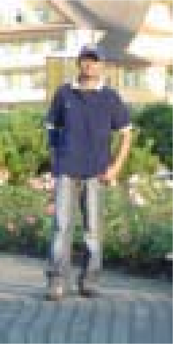
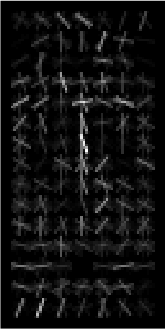
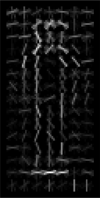
History of Oriented Gradients feature transformation applied on a test image. Left: Test image. Middle: HOG descriptors weighted by positive SVM weights. Right: HOG descriptors weighted by negative SVM weights. Source: .
Introduced in , Histogram of Oriented Gradients (HOG) have been developed as an important improvement over scale-invariant feature transform (SIFT) descriptors. The main idea behind HOG features is that local object shapes and appearances in an image can be expressed as a distribution of color intensity gradients. The above figure shows a test image of a pedestrian in and the HOG descriptors weighted by positive and negative Support Vector Machine (SVM) weights, which were used to classify the presence of a pedestrian, in and respectively. HOG features became an important foundation of many object detectors ; ; , as well as other computer vision tasks.
The peak of traditional object detection methods was reached with the Deformable Part-based Model (DPM) proposed by , winning the VOC-07, -08, and -09 detection challenges. It is built on the foundations of the HOG detector and views training as the task to learn how to decompose an object while inference is an ensemble of detections of different object parts. Detecting a person would then be translated into the decomposed detection of a head, legs, hands, arms, and body, which was also called the “star-model” in . later improved this to “mixture models” ; ; , coping with objects of larger variation.
Deep Learning based Object Detection
After the success of DPMs, improvements in object detectors stagnated. With the comeback of convolutional neural networks (CNN) in 2012, deep architectures have been developed to learn robust and high-level task agnostic feature representations of images that easily superseded hand-crafted ones. Unsurprisingly, the field of object detection has quickly gained new traction due to successful deep models. This section goes into more detail on different approaches which can be grouped into two-stage detectors and one-stage detectors. The former can be split into two steps that divide the candidate region generation and the actual location regression and object classification while the latter implements an end-to-end solution using a single deep neural network.
Two-Stage Detectors
Two-stage object detectors follow a detection paradigm of a separated (1) proposal detection step, where likely object locations are determined and (2) a verification step, where each proposal is classified into one of the possible classes of objects and additionally the proposed location is fine-tuned.
Regions with CNN Features: R-CNN
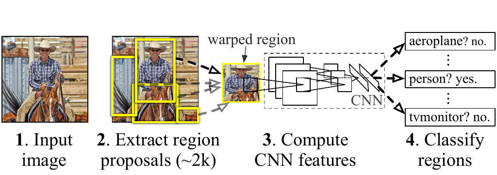
R-CNN object detection system overview. The system (1) takes an input image, (2) extracts region proposals, (3) warps and forwards each proposal through a pre-trained CNN to obtain feature representations and finally (4) classifies each output using class-specific SVMs. Source: .
The first of its kind in the two-stage category of object detectors was R-CNN (Regions with CNN features) by . R-CNN starts with the generation of object proposals that serve as candidates for processing. These are obtained using the selective search algorithm which is a region proposal procedure that computes hierarchical groupings of similar regions based on size, shape, color, and texture. Each object proposal is then warped into a fixed predetermined image size and forwarded through a CNN model, which is pre-trained on ImageNet, to extract a fixed 4096-dimensional feature vector. Afterward, class-specific SVMs perform the object recognition task by scoring each region proposal with their respective class. Finally, a greedy non-maximum suppression is applied, rejecting regions of high IoU values with other regions of the same class achieving higher SVM scores than a learned threshold. The above figure gives a sketch of the inference pipeline. Additionally, the CNN can be fine-tuned on other datasets. To improve the object localization, have applied a separate bounding box regression stage (a similar strategy was introduced in ) that uses class-based regressors to predict new bounding boxes based on the CNN features. R-CNN broke the stagnation in the field of object detection by pushing the VOC07 \(\text{mAP}_{0.5}\) score from 33.7% of DPM-v5 to 58.5%.
Fast R-CNN
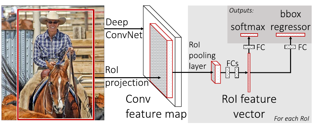
The architecture of Fast R-CNN. The full input image is fed through a CNN to generate feature maps. Based on RoIs, each feature map is pooled into a RoI feature vector and fed into a sequence of fully-connected layers with a classification (object classes) and regression (object localization) head. Source: .
R-CNN was superseded by Fast R-CNN . In Fast R-CNN, the full input images are forwarded through a CNN backbone to produce features maps. For each object proposal output of the selective search algorithm, a region of interest (RoI) pooling layer extracts a fixed-size feature vector from the feature map, inspired by spatial pyramid pooling in SPPNet introduced by . Then, each vector is fed into a sequence of fully-connected layers which then split into two heads, one for softmax classification outputting a probability vector \(\boldsymbol{p}\) of length \(|C|+1\) for the possible classes (with an additional class for the background), and one for the bounding box regression outputting a bounding box offset \(\boldsymbol{t}^{c} = ( t_{x}^{c}, t_{y}^{c}, t_{w}^{c}, t_{h}^{c}, )\) for each of the \(|C|\) object classes (see figure above). To jointly train for classification and bounding box regression, a multi-task loss \(L\) on each labeled RoI is introduced:
\[L\left(\boldsymbol{p}, u, \boldsymbol{t}^u , \boldsymbol{v}\right) = L_{cls}(\boldsymbol{p}, u) + \lambda\left[u \geq 1\right]L_{loc}\left(\boldsymbol{t}^u, \boldsymbol{v}\right) ,\] where \(u\) is the ground-truth label, \(\boldsymbol{v}\) is the ground-truth bounding box regression target, the Iverson bracket indicator function \([u \geq 1]\) evaluates to 1 when \(u \geq 1\) and 0 otherwise, and the hyperparameter \(\lambda\) controls the balance between the two task losses. For classification the binary cross-entropy loss and for bounding box regression, the SmoothL1 loss is used to accumulate over the coordinates. For background RoIs (\(u = 0\)) \(L_{loc}\) is ignored due to missing ground-truth references.
This approach is closer to an end-to-end solution than its predecessors as it gets rid of the multi-stage pipeline and can be trained given only the input image and the object proposals coming from an off-the-shelf algorithm. Fast R-CNN improves training time by a factor of 9 (with a VGG16 backbone) and testing time by a factor of 213, and pushes the \(\text{mAP}_{0.5}\) score on VOC07 to 70.0%.
Faster R-CNN
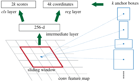
The End-to-end unified architecture of Faster R-CNN including an 'attention' module called Region Proposal Network (RPN) generating likely object proposals (location and objectness) based on $k$ predefined anchor boxes. Source: .
Fast R-CNN was expanded by Faster R-CNN , replacing the external object proposal stage with an end-to-end approach (see figure above). have introduced a so-called Region Proposal Network (RPN) serving as an “attention” model which is a fully convolutional network that takes an image of any size as input and predicts a set of bounding box proposals. Each proposal is attached with an objectness score that measures the membership to a set of object classes against the background class. Instead of generating final bounding box locations of the object proposals, introduce the notion of anchors, making Faster R-CNN the first anchor-based detector. These are used as a baseline reference box for which an offset has to be regressed (see figure above). Anchor-boxes are predefined with different scales (e.g. \(32\times32\), \(64\times64\), …) and aspect ratios (e.g. 1:1, 1:2, 2:1, 5:1, …). For each position in a convolutional feature map in the RPN, a sliding window approach computes a vector of \(2k\) objectness scores, one for the class “object” and one for the class “background”, as well as \(4k\) bounding box offsets where \(k\) is the number of different anchors (the product of the number of anchor scales and the number of anchor aspect ratios). Therefore, the RPN generates \(W \cdot H \cdot k\) proposals, where the intermediate feature map is of size \(W \times H\).
Embedding the region proposal generation into the network stack has improved the VOC07 \(\text{mAP}_{0.5}\) to 73.2% (COCO \(\text{mAP}_{0.5}=42.7\%\), COCO \(\text{mAP}_{\left[0.5, 0.95\right]}=21.9\%\)). Faster R-CNNs therefore became the first end-to-end and the first near-realtime object detector (17fps with a ZFNet backbone). Computational redundancies at the subsequent detection stage have later been reduced in RFCN using fully convolutional networks, and Light-Head R-CNN thinning out the prediction heads and replacing the CNN backbone with smaller networks (e.g. Xception ).
Faster R-CNN has been extended in Feature Pyramid Networks (FPN) . Feature pyramids are a principal component in computer vision tasks for objectives that have to be solved at multiple scales. Until the development of FPN, deep learning-based object detectors have been avoiding feature pyramids, mostly due to their computational complexity and high memory usage. FPNs utilize the inherent multi-scale hierarchy present in deep convolutional networks and introduce feature pyramids with almost no extra cost. Instead of only using the very last output in the convolutional layer sequence, FPNs introduced a top-down architecture with lateral connections (see figure above) which extracts intermediate feature maps from another deep network (in this context called backbone). This architecture allows building high-level semantics at all scales, significantly improving scores on COCO to \(\text{mAP}_{0.5}=59.1\%\) and \(\text{mAP}_{\left[0.5, 0.95\right]}=36.2\%\). Feature Pyramid Networks have since become one of the basic building blocks for many newer object detectors.
One-Stage Detectors
In contrast to two-stage object detectors, a parallel line of development took place with a very different approach. Instead of having a separate stage in the network that proposes where an object is likely, one-stage detectors predict object locations and classes on a grid that can be mapped onto the input image in a single pass which is methodologically simpler and computationally faster. This also allows the object detector to be trained in a simple end-to-end fashion, therefore optimizing the whole network in a unified way towards the defined objective, unlike two-stage methods which usually have to define freezing phases for different network parts with different loss functions to achieve a stable training (see “4-Step Alternating Training” in .
You Only Look Once (YOLO)
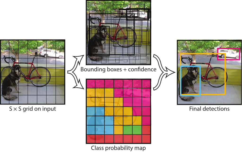
YOLO divides the input image into a grid of $S\times S$ patches. Each grid cell then predicts $B$ bounding boxes, confidences for the boxes, and $C$ class probabilities. Source: .
The most prominent and also first one-stage object detector was YOLOv1, proposed by . The network separates the input image into a grid of \(S \times S\) patches and predicts bounding boxes, object confidences, and class probabilities for each patch at the same time (see figure above), reaching \(\text{mAP}_{0.5} = 63.4\%\) on VOC07. YOLOv1 was improved in YOLOv2 , adapting anchor boxes from Faster R-CNN, achieving a \(\text{mAP}_{0.5}\) score of 78.6% on VOC07, and \(\text{mAP}_{0.5}=44.0\%\) and \(\text{mAP}_{[0.5,0.95]}=21.6\%\) on COCO. It nevertheless suffered from weak localization accuracy for small objects, which was addressed in YOLOv3 by making use of features from multiple scales, similar in concept to feature pyramids in FPNs (\(\text{mAP}_{0.5} = 57.9\%\) and \(\text{mAP}_{[0.5,0.95]} = 33.0\%\) on COCO).
Single Shot Detection (SSD)
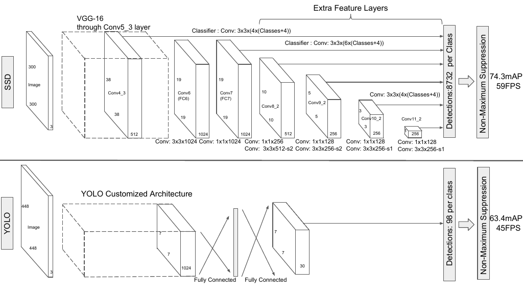
An architectural comparison of SSD (top) and YOLOv1 (bottom). SSD works without any fully-connected layers and adds convolutional feature layers on-top of the backbone network to predict offsets for a set of anchor boxes at multiple feature scales. Evaluated mAP values are for the VOC07 dataset. Source: .
SSD, proposed by , was the second one-stage object detector after YOLOv1. Its major contribution is using default boxes of different scales on different intermediate feature maps instead of only using the last layer (see figure above). Taking multiple feature scales into account, SSD offers advantages in terms of detection speed and accuracy over YOLOv1, especially for small objects (VOC07 \(\text{mAP}_{0.5}=76.8\%\), COCO \(\text{mAP}_{0.5}=46.5\%\), COCO \(\text{mAP}_{\left[0.5, 0.95\right]}=26.8\%\), and a fast version running with 59FPS VOC07 \(\text{mAP}_{0.5}=74.3\%\) depicted in the above figure).
RetinaNet
In RetinaNet , discover that one-stage detectors have trailed two-stage detectors in terms of accuracy due to their unmanaged class imbalance of positive and negative samples. Two-stage detectors can use sampling heuristics such as a fixed foreground-to-background ratio (typically 1:3), or online hard example mining (OHEM) to maintain the class balance between foreground (positive samples) and background (negative samples). Since one-stage detectors perform a single pass and have no stage to filter possible object proposals, they evaluate about \(10^4\) to \(10^{5}\) candidate locations per image while only a few locations contain objects, causing the following two issues: (1) inefficient training since most locations are easy to pick backgrounds and do not contribute any useful learning signal and (2) negative sample numbers overweight positives ones by a large margin, leading to degenerate models as the training can only adjust to few positives in comparison to negatives. To tackle this issue in one-stage detectors, the authors propose the so-called Focal Loss which represents a modified version of the cross-entropy loss. The main idea of Focal Loss is to automatically down-weight the contribution of easy examples during training and focus the model on hard examples with low confidences. Using feature pyramids from FPN (with a ResNeXt-101-FPN backbone) and anchor boxes from Faster R-CNN, RetinaNet managed to beat previous state-of-the-art results with a COCO mAP of 40.8%, surpassing the best one-stage detector DSSD513 (with a ResNet-101-DSSD backbone) at 33.2% mAP as well as the best two-stage detector Faster R-CNN (with an Inception-Resnet-v2-TDM backbone) at 36.8% mAP.
Anchor-Free Object Detection
Although anchor-based methods have shown great success, they come with increased methodological and computational complexity. show in that detection performance is sensitive to anchor box size, aspect ratio and number. Therefore, hyper-parameters need to be additionally tuned to find anchors appropriate for the specific dataset. Moreover, anchor-based detectors have difficulties with objects of large shape variations, as well as small objects. The need for fine-tuning moreover impedes the model’s generalization abilities, as anchors need to be redesigned for new tasks. Most anchor boxes are labeled as negative samples during training since anchors are required to be placed densely on the input image (FPN e.g. places 180k anchors) leading to only a few anchors overlapping with positive samples. Logically, the question of whether anchor-based solutions are the optimal way to solve object detection arises. The recent field of anchor-free object detection tries to find answers to this exact question. First results show, that approaches without object anchors are competitive and capable of beating state-of-the-art anchor-based models, with the advantage of being faster and methodologically less complex.
Early approaches such as DenseBox , the first unified end-to-end fully convolutional detector, UnitBox tackling the localization with an IoU-based loss, YOLOv1 focusing on real-time object detection, were made but without success in surpassing anchor-based systems such as Faster R-CNN at that time.
CornerNet approaches the bounding box prediction by predicting a pair of keypoints, the top-left, and bottom-right corners. The network predicts a heatmap for the top-left corner, a heatmap for the bottom-right corner, and an embedding for each corner which is supposed to group pairs of corners that belong to the same bounding box, minimizing embedding vector distance between pairs. Embeddings are produced using the Associative Embedding technique to separate different instances. CornerNet achieves a mAP of 42.2% on COCO. CenterNet builds on top of CornerNet and includes the prediction of a center keypoint used to perform center pooling. Additionally, CenterNet also introduces cascade corner pooling as an extension to corner pooling from CornerNet which performs max-pooling first along the bounding box borders and then along the orthogonal row/column towards the region center. This addresses the problem that CornerNet and most other one-stage detectors lack an additional look into the cropped regions by exploring the visual patterns within each predicted bounding box. CenterNet achieves a mAP of 47.0% on COCO, giving a significant improvement of 4.8% mAP over CornerNet.
ExtremeNet on the other hand is motivated by who proposed to annotate bounding boxes by marking the objects’ four extreme points: top, bottom, left, right. In ExtremeNet, object extreme keypoints are predicted as follows. First, four multi-peak heatmaps, one for each extreme, are predicted for each object category to generate possible extreme points. Then, each combination between a top, bottom, left, and right extreme point is being generated and their geometric center is being compared to a fifth heatmap that generates center keypoints. If the geometric center is close to one of the peaks in the center heatmap (distance above a fixed threshold), the extreme point combination is valid and an object is predicted.
FCOS uses a fully convolutional one-stage detection approach introducing the notion of center-ness, which depicts the normalized distance from the location to the center of the object that the location is responsible for. The center-ness is used to adjust the classification confidence and thus helps to suppress low-quality detected bounding boxes and improves overall performance by a large margin (\(\text{mAP}_{[0.5,0.95]}\) on the COCO minival validation subset of 37.1% with, compared to 33.5% without the center-ness branch).
FoveaBox is a single unified network, composed of a backbone network and two task-specific sub-networks, following the RetinaNet design. Its main contribution is the assignment of different object scales to different feature pyramid outputs, i.e. each pyramid layer is responsible for a certain interval of object sizes.
Oriented Object Detection
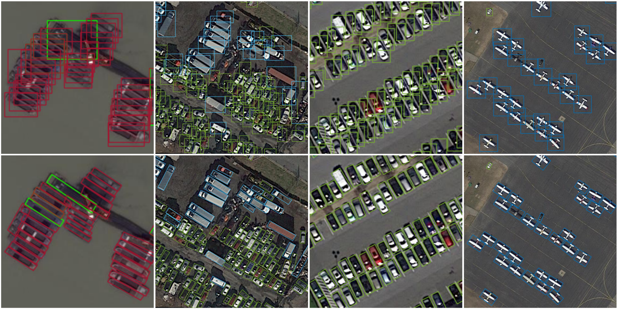
Comparison of axis-aligned (top) and oriented (bottom) bounding boxes in object detection on aerial view imagery. It becomes clear that the oriented bounding box representation is superior for oriented objects and generates tighter boxes that better cover the true area of the object.
Oriented object detection has recently gained more attention in computer vision for aerial imagery, scene text, and face detection. In oriented object detection, bounding boxes are not bound to be strictly horizontal and vertical along the x- and y-axis but can be either rotated by an arbitrary angle or defined by an arbitrary quadrilateral consisting of the four corners. This allows for tighter bounding boxes, especially in densely populated regions as well as for objects that are not parallel to the physical x-y plane, where x is the horizontal and y is the vertical axis. The above figure shows the effect of using oriented bounding boxes, compared to horizontal bounding boxes. The top row shows axis-aligned bounding boxes on ships, vehicles, and airplanes in aerial view imagery while the bottom row shows their respective oriented bounding boxes. It is clear that the oriented bounding box representation is superior for oriented objects and generates tighter boxes that better cover the true area of the object.
Two-Stage Detectors
Since this field has only recently received more attention, current approaches are usually based on methods that are successful in horizontal object detection. A straightforward approach to tackle oriented object detection is to extend the prediction of a bounding box with an additional parameter \(\theta\), determining the rotation angle. did so by using a similar network as Faster R-CNN, expanding the bounding box priors by multi-angle anchors including rotations between 0\(^{\circ}\) and 180\(^{\circ}\), thus increasing the anchor hyperparameter set significantly. Similarly, propose Rotation Region Proposal Networks (RRPN), adapting the Region Proposal Network from Faster R-CNN, designed to generate RoIs with angle rotation information.
Inspired by Mask R-CNN , proposed a semantic segmentation-guided RPN (sRPN) using the atrous spatial pyramid pooling (ASPP) module from to suppress background clutter and a RoI module that fuses multi-level outputs from an FPN. Similarly, SCRDet++ introduced the idea of instance-level denoising on the feature maps into object detection to enhance the detection of small and cluttered objects, common in satellite images.
RoI Transformer is another two-stage anchor-based detector where the geometric transformation from horizontal bounding boxes to oriented bounding boxes is learned and applied to the RoI output of an RPN, such as in Faster R-CNN.
argue that a five-point representation of oriented bounding boxes can cause training instability as well as performance decreases. They ascribe this to the loss discontinuity which results from the natural periodicity of angles and therefore possible exchanges of width and height in the box representation. To circumvent this discontinuity, propose to use the quadrilateral representation in combination with a loss modulation that greedily minimizes the loss from the set of possible edge assignments.
One-Stage Detectors
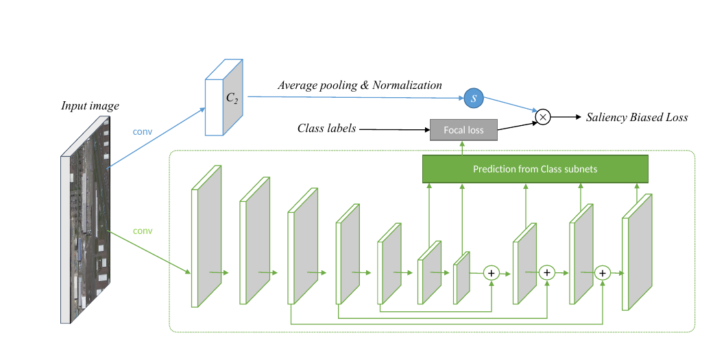
Salience Biased Loss model architecture. The lower network part (green) is the RetinaNet backbone generating multiscale feature maps while the upper part (blue) is a second network which estimates the salience maps used to adapt the focal loss to the difficulty of the current image. Source: .
Similar to , propose a novel loss function based on salience information directly extracted from the input image. Like the Focal Loss, the proposed Salience Biased Loss (SBL) treats training samples differently according to the complexity (saliency) of an image. This is estimated by an additional deep model trained on ImageNet in which the number of active neurons across different convolution layers are measured (see figure above):
\[S = \frac{1}{C \cdot W \cdot H} \sum_{c=1}^{C} \sum_{w=1}^{W} \sum_{h=1}^{H} f\left( \boldsymbol{x} \right)_{c,w,h} ,\] where \(S\) is the average activation value across the layer and \(f\) is a convolution operation with an output feature map of size \(C \times W \times H\). The idea is that with increasing complexity, more neurons will be active. The saliency then scales an arbitrary base loss function to adapt the importance of training samples accordingly.
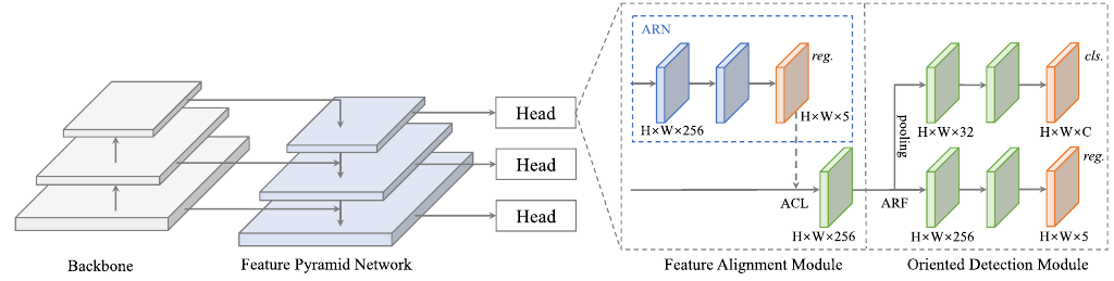
Architecture illustration of S2A-Net consisting of a backbone pretrained on ImageNet, the Feature Pyramid Network to extract multiscale features, the Feature Alignment Module to generate oriented anchors using aligned convolutions and the Oriented Detection Module using Active Rotating Filters. Source: .
Han et al. approach to solve the discrepancy of classifications score and localization accuracy and ascribe this issue to the misalignment between anchor boxes and the axis-aligned convolutional features. Hence they propose two modules (see the figure above for the full architecture): The Feature Alignment Module (FAM) generates high quality oriented anchors using their Anchor Refinement Network (ARN) and adaptively aligns the convolutional features according to the generated anchors using an Alignment Convolution Layer (ACL).
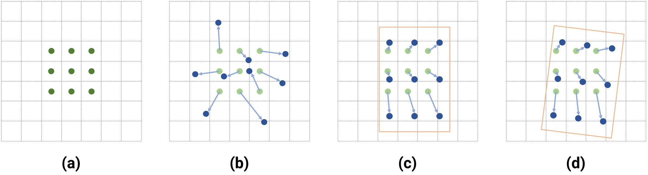
Sampling locations of different convolution operations using a $$3 \times 3$$ kernel. Figure (a) is the default convolution while (b) portrays deformable convolutions , enabling learnable sampling offsets for each of the 9 locations. Figure (c) and (d) are aligned convolutions (AlignConv) which in turn are deformable convolutions but restricted to a global translation, rotation and scaling w.r.t. the full sampling window and are supposed to align the convolution operation to oriented anchor boxes. Source: .
The ACL is a restricted Deformable Convolution Layer in the sense that it learns the same translation, scaling, and rotation for each sampling location (see figure above). The second proposed module is the so-called Oriented Detection Module (ODM). Introduced in Oriented Response Networks (ORN) , make use of Active Rotating Filters (ARF) which is a $k \times k \times N$ convolutional filter that rotates the features $N - 1$ times, generating an output feature map of \(N\) orientation channels, thereby encoding \(N\) orientations directly into the feature maps.
In , the authors tackle the issue of discontinuous boundary effects on the loss due to the inherent angular periodicity and corner ordering by transforming the angular prediction task from a regression problem into a classification problem. They devise the Circular Smooth Label (CSL) technique which handles the periodicity of angles and raises the error lenience to adjacent angles.
One-Stage Anchor-Free Detectors
The following contributions go one step further and remove the concept of anchors, generating predictions on a dense grid over the input image.
IENet is based on the one-stage anchor-free fully convolutional detector FCOS. The regression head from FCOS is extended in IENet by another branch that regresses the bounding box orientation, using a self-attention mechanism that incorporates the branch feature maps of the object classification and box regression branches.
Axis-Learning also builds on the dense sampling approach of FCOS and explore the prediction of an object axis, defined by its head point and tail point of the object along its elongated side (which can lead to ambiguity for near-square objects). The axis is extended by a width prediction which is interpreted to be orthogonal to the object axis.
In PIoU the authors argue, that a distance-based regression loss such as SmoothL1 only loosely correlates to the actual IoU measurement, especially in the case of large aspect ratios. Therefore, they propose a novel Pixels-IoU (PIoU) loss, which exploits the IoU for optimization by pixelwise sampling, improving detection performance on objects with large aspect ratios dramatically.
P-RSDet replaces the Cartesian coordinate representation of bounding boxes with polar coordinates. Therefore, the bounding box regression happens by predicting the object’s center point, a polar radius, and two polar angles. Furthermore, to express the geometric constraint relationship between the polar radius and the polar angles, a novel Polar Ring Area Loss is proposed.
An alternative formulation of the bounding box representation is defined in O2-DNet . Here, oriented objects are detected by predicting a pair of middle lines inside each target, showing similarity to the extreme keypoint detection schema proposed in ExtremeNet.